


When we die, our bodies become rigid (rigor mortis sets in). Niderkorn's (1872) observations on 113 bodies provides the main reference database for the development of rigor mortis and is commonly cited in textbooks. Via a series of log transformations I was able to fit a lovely model to this somewhat unlovely data, for the proportion p(t) of bodies in rigor mortis after t hours. It is illustrated in the graph below: the general two-parameter model that I tried is
![]()
I don't know how I thought of this, except that we'd been looking at models of compositions with exponentials, and I had a feeling that this sort of model might work. Model building is a mysterious and black art. What model might you propose? Models are often compared against each other based on the number of parameters they require, how much predictive power they have, whether they make intuitive sense, whether the parameters are interpretable, etc.
There are log transformations that nearly permit our problem to be resolved using linear regression. Let's proceed as follows:
![]()
and then
![]()
(where we take the negative to the other side because the proportion p(t) itself is between 0 and 1, which means that the first log gives a negative - and the second log would not be defined otherwise for negatives).
We can use our data and linear regression to estimate the parameters, if we define ``new data'' from the old via
So we log-transform the hours, and do two log-transforms of the cumulative
proportion data , after which linear regression is performed
to get the estimated parameters. This process is encoded in xlispstat as
follows:
, after which linear regression is performed
to get the estimated parameters. This process is encoded in xlispstat as
follows:
(setq
  hours '(2 3 4 5 6 7 8 9 10 11 12 13)
  bodies '(2 14 31 14 20 11 7 4 7 1 1 2)
  ;; there are a total of 114 bodies
  cumulatives '(2 16 47 61 81 92 99 103 110 111 112 114)
  proportions (/ cumulatives 120)
  ;; new we perform linear regression (with intercept):
  reg (regress (list (ln hours)) (ln (- (ln proportions))))
  ;; and ask reg for its coeficients:
  coefficients (send reg :coef-estimates)
  )
which resulted in the coefficients (and hence the model)
![]()
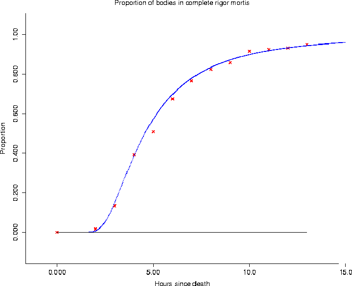
Figure 1: The linear regression results.
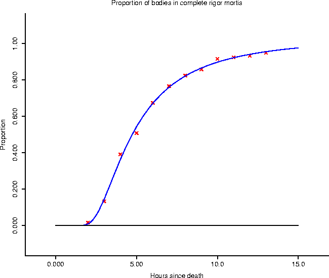
Figure 2: The non-linear regression results appear to be a slight improvement.
Now we'd like to compare our result with that obtained using non-linear regression. One of the advantages of non-linear regression is that the ad hoc choice of 120 as the number of bodies to divide by is eliminated by estimation of a multiplicative constant in front of the model:
![]()
where c is the cumulative number of bodies in rigor mortis at time
t, and ![]() is a multiplicative constant (which we'll guess is about 120,
to start). The other parameters are estimated by their values from linear
regression.
is a multiplicative constant (which we'll guess is about 120,
to start). The other parameters are estimated by their values from linear
regression.
Here is the xlispstat code which implements this procedure:
;; initial values (solutions of linearization)
(setq
 gamma 120
 alpha (exp (first coefficients))
 beta (- (second coefficients))
 nreg (nreg-model
      (lambda(theta)
	(let (
	      (gamma (elt theta 0))
	      (alpha (elt theta 1))
	      (beta (elt theta 2))
	      )
	  (* gamma (exp (- (/ alpha (^ hours beta)))))
	  )
	)
      (cumsum bodies)
      (list gamma alpha beta)
      )
 )
Residual sum of squares: 47.4054
Coefficients: (124.382 19.424650502192684 2.127669245585588)
Residual sum of squares: 40.9828
Coefficients: (124.42338726758184 21.334959045370884 2.1745553351139515)
Residual sum of squares: 40.7887
Coefficients: (124.3834661473006 21.518819388090982 2.177378350279522)
Residual sum of squares: 40.7887
Coefficients: (124.3819389982478 21.522880354505403 2.1774842047896654)
Residual sum of squares: 40.7887
Coefficients: (124.38193962238628 21.522890934820094 2.1774844349107663)

Least Squares Estimates:

Parameter 0                124.382      (2.87169)
Parameter 1                21.5229      (3.99613)
Parameter 2                2.17748      (0.140507)

Sigma hat:                 2.12887
Number of cases:                12
Degrees of freedom:              9