Linear functions can be used as models in the biological sciences when a particular dependent quantity changes at a constant rate with respect to an independent variable. From a modeling perspective, the equation, y (x) = mx + b, can be interpreted as follows,

There are many linear models in the life sciences. We will introduce the basic concepts of linear modeling by considering linear growth models.

Linear Growth Model

Organisms generally grow in spurts that are dependent on both environment and genetics. Under controlled laboratory conditions, however, one can often observe a constant rate of growth. These periods of constant growth are often referred to as the linear portions of the growth curve. In this example, we will construct a linear equation to model the linear phase of growth for a hypothetical insect larvae.

Suppose the larvae of a particular insect species grow linearly in mass during the last instar, from t = 0 to t = 48 hours. Laboratory observations indicate that, on average, the larvae are initially 8 grams and grow to an average size of 12 grams over the 48 hour period. To find the equation that models the growth, we must find the constants m and b in the equation,

The variable y represents larval mass in grams (g) and t represents time in hours (h). We place the restriction 0 ≤ t ≤ 48 on t because the model is only valid from hour 0 to hour 48. At hour 48, growth will begin to slow as the insect prepares to undergo pupation. Therefore, our model is only valid for the linear portion of the growth curve.

Now that we have our model, we can find the initial mass of the larvae (represented by the constant b) based on the information provided. We are given that the larvae are initially 8 g, therefore b is equal to 8 and we write,

y = mt + 8.

To find the slope of the line (m), we take two points that we know to lie on the line. We choose the two points as (t₁, y₁) = (0, 8) and (t₂, y₂) = (48, 12) based on the information given. Using the formula for slope, we have,

Therefore, we can write the equation that models larval insect growth as,

Now that we have dealt with the numbers and variables, we must also make sure our model has consistent units. The units on each side of the equation must match- the dependent variable on the left side of the equation has units of grams, then the units on the right side must also be grams. Checking the consistency of the units is called dimensional analysis.

There are two terms on the right hand side, mt and b. Both of these terms must have units of g. Naturally, the term b, which represents the initial mass of the larvae, has units of g; and t, which represents time, has units of hours. What are the units on m? We can determine m’s units as follows,

where · represents m’s units. Using this equation, we see that · must have units of g/hour in order for hours to cancel as,

Thus, we interpret our slope using the units as:

“Larvae grow 1 /12 th of a gram per hour.”

Of course, our model is only an approximation to reality; there will exist variation in mass among larvae. For example, one larva may grow to 12.1 g while another grows to only 11.9 g over the 48 hours. We simply know that on average a larva grows to 12 g over the 48 hour time period.

Population Growth Rate

Linear models can also be applied to the growth of a population of organisms. For example, the logistic population growth model assumes that the population growth rate (r) decreases linearly with population size (N) through a process known as intraspecific competition. The population growth rate can be positive, negative, or zero. If r is greater than zero the population grows, while if r is less than zero the population declines. When r = 0 the population size remains constant.

We can write an equation for r as a function of N as follows,

where r₀ > 0 is the population growth rate in the absence of intraspecific competition and
K > 0 is the carrying capacity of the environment. We can rewrite r(N) in slope-intercept form as,

In this example, the dependent variable is the population growth rate, r , and the independent variable is the population size, N, since r₀ and K are positives numbers. The slope of the line is given by

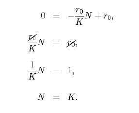
the negative sign indicates that r decreases with N. The r-intercept (y-intercept) is given by b = r₀ , which means that when N = 0, there is no intraspecific competition. We can find the N-intercept (x-intercept) of r (N) by setting r (N) = 0 and solving for N,

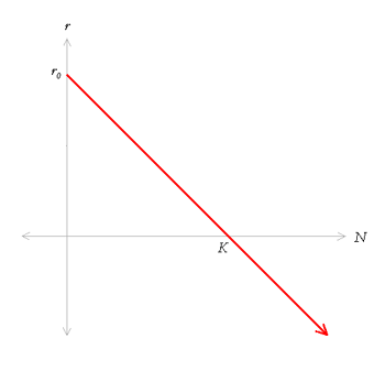
Therefore, we find the N-intercept to be K. We set r (N) equal to zero as above because the r-coordinate (y-coordinate) of points lying on the N-axis (x-axis) must be zero. We can plot r(N) as follows,

This graph indicates that

In other words, the population grows when the population is below the carrying capacity, and declines when the population is above the carrying capacity. When the population size is at the carrying capacity ( N = K), there is no growth or decline (r = 0) .

*****

In the next section we will examine some other applications of linear models.

Applications