- Exercises p. 226, #4, 5
Begin with Exercise #3, p. 226:
- R2: a measure of fit
- See figure 4.5, p. 158
- R2 represents the amount of variation explained by the model against a constant model (using the mean: y=ybar). Recall this model from last time in several plots (the shotgun blast, the horizontal line).
- "Some books call R2 the coefficient of determination" (p. 159)
- Hint for Exercise #2, p. 226 (based on "trick" from last time)
- Finding R2 in the non-linear case
- same as R2 in the linear case!
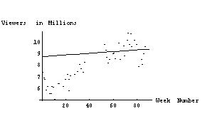
- Example - the X-files (using results from Mathematica)
- Typical use of regression: predict year two's results from year one's results
- Discussion of the "failures" of the process
- Using the model of the first season with the data of the second season results in a higher R2! Linear regression minimizes the Residual Sum of Squares, rather than maximizing R2.
- Season two would have done a woeful job of predicting year
one:
- Curvilinear models
- Catalog of functions - standard classes:
- ladder of powers
- exponential and log
- trigonometric (periodic) functions
- Intrinsically linear models - parameters are linear
- Linearizable models - parameters enter in a non-linear way, but data may be transformed to yield linear procedure
- Catalog of functions - standard classes:
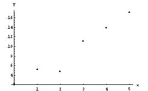
- Example: Cost of advertising. Comparison of various models:
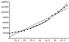
- linear model
- log-linear (i.e. exponential linearizable model)
- log-log model (i.e. power linearizable model)
- If ever there were a data set crying out to be modeled as a logistic, this is the one! Notice that nice inflection point. The logistic, however, is not linearizable, as we see in the bear data example.
- Examples:
- Lynx data:
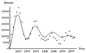
- Long term trend: horizontal asymptote (perhaps zero!)
- Decaying oscillations (some periodicity)
- Model: exponential decay to steady value (1,934 here), with decaying oscillations of ten-year period.
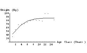
- Bear data - intrinsically non-linearizable model: the logistic
-
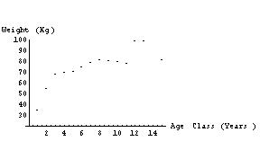
- long term trend: horizontal asymptote
- concave down? Increasing with decreasing slope....
- positive y-intercept
- model: logistic
- "With nonlinear problems such as the logistic, choosing good [initial parameter] guesses is essential." (p. 183)
-
- Lynx data:
Notes:
- In the end, the result is to be a model. The question then becomes one of interpretability: can the model that results explain? Or is it simply a way of predicting values that are close to the actual, without any sort of knowledge being gained? We certainly hope that knowledge increases, based on the model that results.
- Mathematica file to generate these figures and models
Some Questions:
- What is the range for which the model might remain valid? How far can you trust this model (how far can you throw this model)?
- When is complexifying worthwhile? How do I decide whether R2 is okay?