BioMath: Linear Functions

Linear Functions

The Basics

To understand linear relationships in biology, we must first learn about linear functions and how they differ from nonlinear functions.

Definition: Linear and Nonlinear Functions

The key feature of linear functions is that the dependent variable (y) changes at a constant rate with the independent variable (x). In other words, for some fixed change in x there is a corresponding fixed change in y. As the name implies, linear functions are graphically represented by lines.

Definition: A linear function is a function that has a constant rate of change and can be represented by the equation y = mx + b, where m and b are constants. That is, for a fixed change in the independent variable there is a corresponding fixed change in the dependent variable.

If we take the change in x to be a one unit increase (e.g., from x to x + 1), then a linear function will have a corresponding constant change in the variable y. This idea will be explored more in the next section when slope is discussed.

Nonlinear functions, on the other hand, have different changes in y for a fixed change in x.

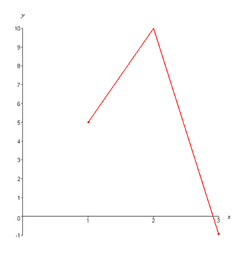
Definition: A nonlinear function is a function that is not linear. That is, for a fixed change in the independent variable, there is NOT a corresponding fixed change in the dependent variable.

The following graph depicts a nonlinear function with a non constant rate of change,

In this example, there is both a 5 unit increase in y and a 11 unit decrease in y corresponding to a one unit increase in x. A nonlinear function does not exhibit a constant rate of change, and therefore is not graphically represented by a line. In fact, you probably think of nonlinear functions as being curves. The following table summarizes some of the general differences between linear and nonlinear functions:

Linear Functions

Domain and range is all real numbers.

Graphically represented by a straight line.

Nonlinear Functions

Domain and range can vary.

Often graphically represented by a curve.

Representing linear functions

Linear functions can be written in slope-intercept form as,

y(x) = mx + b.

We can use the slope-intercept form of a line to demonstrate that a linear function has a constant rate of change. To see this, consider a one unit increase in x (i.e. from x to x + 1). According to our linear equation, a one unit increase in x results in,

y (x + 1) = m(x + 1) + b = mx + m + b.

Examining the difference in the y values for a one unit increase in x gives,

y (x + 1) − y (x) = mx + m + b − (mx + b) = m.

That is, a one unit increase in x corresponds to an m unit increase or decrease in y, depending on whether m is positive or negative.

*****

In the next section we will explore the concept of slope.

Slope