Graphing Exponential Functions
As an experimental scientist you would start with the data, as we did in the examples of cancer incidence and viral decay, determine that the trend is exponential, and then find the best mathematical model to fit your data. However, it is often easier to understand different models if we consider the idealized curves. To better understand the features of exponential growth and decay, we will consider some general exponential functions through a mathematicians eyes.
Consider the following two exponential functions:

Let's construct a table of values for f1 (x) and f2 (x) to use as a guide when plotting.
|
x
|
- 4
|
-3
|
-2
|
-1
|
0
|
1
|
2
|
3
|
4
|

|
16
|
8
|
4
|
2
|
1
|
1/2
|
1/4
|
1/8
|
1/16
|

|
1/16
|
1/8
|
1/4
|
1/2
|
1
|
2
|
4
|
8
|
16
|
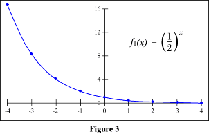
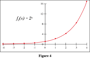
We can then plot the points listed in table above and draw a
smooth curve through all of them.

|

|
| Let's discuss some of the features of these graphical
representations. |
| Exponential
Decay
0 < a < 1
Properties
- As x → ∞, f1 (x) → 0
This means the curve decrease
as you look to the right because f1 (x) approaches
the y = 0 (properly
called the horizontal
asymptote).
- As x → - ∞, f1 (x) → ∞
In other words the curve
increases without bound to the left.
- If x =
0, f1 (x)
= 1
The curve intersects the y-axis
at the point (0, 1). This point is called the y intercept.
|
Exponential
Growth
a > 1
Properties
-
As x → ∞, f2 (x) → ∞
An exponential growth curve
increases without bound as you look to the
right because the value of f2 (x) increases
as x increases.
-
As x → - ∞, f2 (x) → 0
The curve decreases as you look
to left because the value of f2 (x) approaches
the horizontal asymptote, y = 0.
-
If x =
0, f1 (x) = 1
The curve intersects the y-axis
at the point (0, 1). This point is called the y intercept.
|

You can verify the accuracy of the curves
we have just drawn using a graphing calculator or
program.
|
Notice that f1 (x) and f2 (x) exhibit
contradictory behavior. In general any exponential function, y = a x,
will look similar to either
 or or  , ,
depending on whether a is less than
or greater than one respectively.
Constructing graphs of other exponential functions.
Now that we have constructed graphs for f1 (x) and f2 (x) and discussed their
general characteristics, you may be wondering how to construct
graphs of other exponential functions.
When plotting exponential functions it is imperative to determine
whether you are working with exponential growth or decay. You
can determine this by looking at the base of a function you
are given or by the nature of the application. For example,
if you a plotting the growth of a culture of bacteria growing
under ideal laboratory conditions, you would expect to see an
exponential growth curve. However, if you are interested in the decay of a radioisotope, you would expect an exponential decay curve.

When you are confused, it is always useful to construct a table of values for the function in
question. This table coupled with your own intuition about the
shape of the graph should give you a reasonably accurate sketch
of the function in question.
*****
In the next section we will look at slightly more complicated
variants of our basic exponential
function, y = a x.
|


