|
|
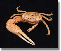
Image
used with permission of
Southeastern Regional Taxonomic
Center
(SERTC), South Carolina
Department of Natural Resources. |
If you never thought that sex appeal could
be calculated mathematically, think again.
Male fiddler crabs (Uca
pugnax) possess an enlarged major claw for fighting or
threatening other males. In addition, males with larger claws attract
more female mates.
The sex appeal
(claw size) of a particular species of fiddler crab is
determined by the following
allometric equation:
Mc = 0.036 · Mb 1.356,
|
where Mc represents the mass of the major claw
and Mb represents the body mass of the crab
(assume body mass equals the total mass of the crab minus the
mass of the major claw)
[1] . Before we discuss this equation in detail, we will define and discuss allometry
and allometric equations.
|
What is Allometry?
Allometry is the study of the relative change in proportion
of an attribute compared to another one during organismal growth.
These attributes may be morphological, physiological, or otherwise.
A well known example of an allometric relationship is skeletal
mass and body mass. Specifically, the skeleton of a larger organism
will be relatively heavier than that of a smaller organism. Of
course it seems obvious that heavier organisms require heavier
skeletons. But is it equally clear that heavier organisms requires disproportionately heavier skeletons? So how does the relationship work? Consider the following data:
- a 10 kg organism may need
a 0.75 kg skeleton,
- a 60 kg organism may need a 5.3 kg skeleton, and
yet
- a 110 kg organism may need a 10.2 kg skeleton.
As you can see by inspecting
these numbers, heavier bodies need relatively beefier skeletons
to support them. There is not a constant increase in skeletal
mass for each 50 kg increase in body mass; skeletal mass increases
out of proportion to body mass [2].
Allometric scaling laws are derived from empirical data. Scientists
interested in uncovering these laws measure a common attribute,
such as body mass and brain size of adult mammals, across many
taxa . The data are then mined for relationships from which equations
are written.
Allometric Growth
| Allometric scaling relationships can be described
using an allometric equation of the form, |
| |
f (s) = c s d,
|
(1)
|
| where c and d are constants.
The variables s and f (s) represent
the two different attributes that we are comparing (e.g.,
body mass and skeletal mass). |
This equation can be used to understand the relationship between
two attributes. Specifically, the constant d in
this model determines
the relative growth rates of the two attributes represented
by s and f (s). For simplicity, let's
consider the case d > 0 only.
- If d > 1, the attribute given by f (s)
increases out of proportion to the attribute given by s.
For example, if s represents body size, then f (s)
is relatively larger for larger bodies than for smaller bodies.
- If 0 < d < 1, the attribute f (s)
increases with attribute s, but does so at a slower rate
than that of proportionality.
- If d = 1, then attribute f (s) changes
as a constant proportion of attribute s. This special
case is called isometry, rather than allometry.
Using Allometric Equations
Notice
that (1) is a power function not an exponential equation
(the constant d is
in the exponent position instead of the variable s).
Unlike other applications where we need logarithms to help
us solve the equation, here we use logarithms to simplify
the allometric equation into a linear equation.
Here's
how it works
We rewrite (1) as
a logarithmic
equation of the form,
|
| |
log (f (s)) = log (c s d).
|
(2)
|
Then, using the properties of logarithms, we can
rearrange (2) as follows,
|
| |
log (f) |
= log c + log (s d),
|
|
| |
|
= log c + d log s.
|
(3)
|
When we change variables by letting,
|
| |
y |
= log f,
|
|
| |
b |
= log c,
|
|
| |
m |
= d,
|
|
| |
x |
= log s. |
|
you can see that (3) is in fact the linear equation |
| |
y |
= mx + b.
|
(4)
|
Therefore, transforming an allometric equation
into its logarithmic equivalent gives rise to a linear equation.
Why Bother?
By rewriting the allometric equation into a logarithmic equation,
we can easily calculate the values of the constants c and d from
a set of experimental data. If we plot log s on the x-axis
and log f on the y-axis, we should see a line with
slope equal to d and y-intercept
equal to log c. Remember, the variables x and y are
really on a logarithmic scale (since x = log s and y = log f).
We call such a plot a log-log plot.

Because allometric equations are derived from empirical
data, one should be cautious about data scattered around
a line of best fit in the xy-plane of a log-log
plot. Small deviations from a line of best fit are actually
larger than they may appear. Remember, since the x and y variables
are on the logarithmic scale, linear changes in the output
variables (x and y) correspond to exponential
changes in the input variables (f (s) and s).
Since we are ultimately interested in a relationship between f and s,
we need to be concerned with even small deviations from
a line of best fit.
|
Now let's go back to our fiddler
crab as a concrete example.
|
[1] |
McLain, D.K., Pratt, A.E., and A.S. Berry
(2003). Predation by red-jointed fiddler crabs on congeners:
interaction between body size and positive allometry of
the sexually selected claw. Behavioral Ecology 14: 741-747 |
|
[2]
|
Nielsen-Schmidt, K. (1984). Scaling. Why is Animal
Size So Important? Cambridge University Press, Cambridge. |
|