LEAPS & CREEPS: SPATIAL DIFFUSION OF DISEASE

The outline of the module is as follows:

1. Readings: an overview
2. Motivation: spread of a disease through a population

1. Logistic growth
2. Social gravity
3. Geographic concentration of population
4. Barriers to geographic spread

1. Modeling geographic diffusion: the pieces of the puzzle

1. Contagion geographic processes
2. Hierarchical geographical processes
3. Mean information fields

1. Diffusion waves
2. Applications: diffusion of cholera simulation game
3. Summary

I. Readings

This module assumes that you have read

Smallman-Raynor, Matthew and Andrew D. Cliff. The Philippines insurrection and the 1902-4 cholera epidemic: Part I -- Epidemiological diffusion processes in war Journal of Historical Geography, Vol. 24, No. 1. January 1998, pp. 69-89.

A supplemental reading for the interested student is

Smallman-Raynor, Matthew and Andrew D. Cliff. The Philippines insurrection and the 1902-4 cholera epidemic: Part II -- Diffusion patterns in war and peace, Journal of Historical Geography, Vol. 24, No. 2. January 1998, pp. 188-210.

What do we learn from this historical case study about the spread of an infectious disease, namely cholera? Both hierarchical and contagious components played a role in the diffusion of this disease, albeit an unbalanced one. Where a well-developed urban hierarchy exists, hierarchical rather than geographic contagion effects are likely to dominate the diffusion of an infectious disease. Contagion effects are most conspicuous temporally around epidemic peaks.

• The data base used is the 50 weekly recorded incidences of cholera in over 440 settlements geographically distributed across the 7100 islands of the Philippines archipelago, during March 1902 through February 1903.

• Natural isolation (the sea separating islands, and rugged terrain and mountains dissection islands themselves) served as an effective barrier to the spread of infectious diseases.

• Because the Philippine Islands lacked the conditions necessary to maintain cholera in endemic form, the epidemic had a discrete and definable starting point that ended with a subsequent disease-free period.

• REGRESSION ANALYSIS. The time-ordered sequence of appearance of cholera in the settlements of the Philippine Islands urban system was modeled as a function of: (1) urban population size, representing the hierarchical component in the diffusion process; and, (2) geographic distance from the settlement of initial introduction, representing the contagious component in the diffusion process.

• REGRESSION RESULTS.

1. Markedly positive association between distance and time to infection: municipalities proximal to Manila (the point of cholera introduction) tended to be infected first, with more distant centers tending to be infected at increasingly later dates.
2. All seven islands and two-thirds of the provinces display a positive association between distance and time of first infection.
3. A weak association between population size and time to infection: a tendency for larger municipalities to be infected first.
4. Only three provinces displayed a purely hierarchical process; these regions housed the most developed urban hierarchies.

• IMPLICATION. Wave I of the cholera epidemic spread through the archipelago as a mixed diffusion process, with the contagious component being dominant. This is observable at all spatial scales.

• Of note, the rank-size rule (i.e., log-normal distribution) was used to analyze the degree of urban hierarchy development.

• SPATIAL AUTOCORRELATION ANALYSIS IMPLICATIONS.

1. From the start of each local epidemic wave until shortly after the peak week, spatially contagious spread was more important than hierarchical spread.
2. Contagious spread was most important around the peak week.
3. Hierarchical spread was generally most important from two or three weeks before, through six or seven weeks after epidemic peaks.

• PUBLIC HEALTH POLICY IMPLICATION. The reconstruction of this epidemic highlights the ineffectual nature of many of the early counter-measures taken to control the diffusion of cholera.

II. Motivation

Humans and their experiences exist in both space and time--a statement so obvious that many researchers may feel it goes without say. Two penetrating questions arise from this statement, though: (1) How do spatial patterns evolve over time? (2) How do the underlying geographic structures help mold this evolution?

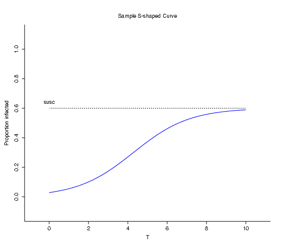
Plotting the cumulative percentage of communicable disease cases against time almost always results in a curve that resembles and thus can be described as being S-shaped. Generally speaking, such a curve arises because frequently there are few cases when a disease first appears. As people interact in a geographic landscape, the disease diffuses. As more people contract the disease, the number having it while interacting increases. As the number of susceptible people contracting the disease increases, the number of uninfected people must necessarily decrease, since there is a fixed total population inhabiting a given geographic landscape. Hence, as time passes, the chance of a disease carrier interacting with an unexposed person decreases. Therefore, in the beginning, when a disease first appears, the total number of cases begins to increase at an explosive rate. But at some point in time, when the chance of interacting with an unexposed person is less than the change of interacting with an exposed person, the rate of increase in the number of cases begins to decrease. Eventually either all, or nearly all, susceptible people are infected, and the disease subsides. An example plot of this type of curve appears in Figure 1:

Of note is that the incubation period for a given communicable disease impacts upon the steepness of the affiliated S-shaped curve. In addition, natural and artificial immunization, and natural resistance to a disease impacts upon the percentage of a population that can contract the disease.

This S-shaped curve can be described with the following equation

percentage of population infected = ,

Rapid diffusion will have a very large value; sluggish diffusion will have a value closer to 0. Effective interventions should reduce the percentage of a population that is susceptible, and should reduce the value, causing the curve to have a more shallow slope.

A plot of the expansion of a disease to new locations also will tend to yield a logistic curve.

Just as the cumulative number of cases displays a systematic pattern through time, the spatial interaction giving rise to diffusion of a communicable disease also displays pattern. This pattern can be described as follows:

where K is a constant of proportionality, _j indexes the relative importance of the origin (o)/destination (d) locations, and is the rate of distance decay.

In other words, the chance of people in two locations interacting decreases as distance separating these locations increases, and increases as the number of people residing at each location increases. Because a diffusion mechanism has some disease going from an origin, where it is present, to a destination, relatively speaking the parameters K and ₁ are unimportant. Moreover, for diffusion from a particular origin (o), the revised equation of interest becomes

In terms of diffusion, if ₂ = 0 and > 0, then a diffusion process is governed solely by distance and is know as contagion diffusion. If ₂ > 0 and = 0, then a diffusion process is governed solely by size of a place and is known as hierarchical diffusion, principally because places are organized in geographic space according to some hierarchical structure. If ₂ = 0 and = 0, then a diffusion process is random; this situation is rare.

Of note is that population and distance can be measured in different ways.

Population tends to concentrate in space, with these concentrations today being cities, towns, villages, and hamlets. These urban places often are organized in space, in terms of number, size and spacing, according to economic principles. These economic principles, as well as administrative principles and needs of transportation networks, yield hierarchical structurings of urban places. For example, county health departments may be located in county seats, and report to state health departments, which may be located in state capitals, which in turn report to federal health agencies, which may be located in the national capital. This hierarchical structuring may be visualized as pyramidal in shape, reflecting the greater number of smaller urban places (the pyramid's base) and the decreasing number of increasingly larger urban places (moving toward the pinnacle at the top of the pyramid). One feature of this hierarchical organization of urban places is that as position in a given hierarchy increases, population tends to increase. This regularity in the concentration of population within a geographic landscape is why the spread of a communicable disease dominated by population size is referred to as hierarchical diffusion.

A second generalization concerning the number and size of urban places is based upon an empirically established rule. This rule has been derived from the relative distribution of total population for a large region or a nation across its urban places. When a set of urban places is ranked in descending order on the basis of size, the resulting size-distribution of population may be described as follows:

population of urban place having rank r = ,

where r is an integer indicating the rank of the i-th urban place, and is a parameter indicating the nature of the average slope of a scatterplot trend line for LN(population_r) versus LN(rank)--a log-log scatterplot. Therefore, once the population of the largest city in a large region or country is measured, and if the value of is known, then it becomes possible to calculate the population of an urban place of any rank. Many explanations have been posited concerning why this equation repeatedly furnishes such a good description of the size distribution of urban places; none are universally accepted, though. Zipf, one of its first proponents, set = 1, and interpreted the rule as a reflection of unifying, centralizing power. Later social scientists interpreted this rule as the outcome of the law of entropy (i.e., a circumstance in which forces affecting the size distribution are many and act randomly); a lognormal distribution is the limiting, equilibrium case of a stochastic growth process. In other words, an ideally balanced and well-integrated urban hierarchy has been achieved, absent of virtually any influence of strongly deforming forces, when the rank-size rule prevails.

The city size distributions derived from rank-size and central place principles are compatible, confirming that the rank-size distribution is hierarchical. But not only its log-log slope, but also the degree of descriptive precision accompanying this equation is important. As the slope, , approaches 1 (i.e., the log-log plot conforms to a straight line with a slope of -1), a well-integrated regional/national system of cities is achieved. Accordingly, the estimated value of sometimes is used to index the degree of development of an urban hierarchy (for instance, see Smallman-Raynor and Cliff). Of note, and in contrast, as the gap between the first and second cities in this log-log plot increases (i.e., is a poor predictor of the size of the second-largest urban place), primacy prevails and the population of a nation or large region is tending to concentrate in a single city; multimodal variants of primacy are possible, too.

For illustrative purposes, consider the geographic distribution of population across Puerto Rico's 78 municipalities, each focusing on an urban place. AIDS has diffused to the island from New York City, first appearing in San Juan, the largest city on the island. A rank-size rule description of the distribution of population across the island's municipalities, based upon 1998 population estimates, is furnished by

population of island's municipality at rank r = , R² = 0.986,

where 439,427 is the population of San Juan. Overlooking measurement error (e.g., the population of a municipality and its principal city are not exactly the same), the value of 0.7 suggests that the island's urban system is not fully integrated. Consequently, hierarchical diffusion mechanisms should be less effective, as has been the case with the diffusion of AIDS across the island.

While economic, political and/or social principles might establish conditions for a hierarchical organization of urban places in geographic space, mechanisms for generating them and reinforcing their existence merit discussion, too. Although governmental administrative roles constitute one mechanism, producing a county-state-national structure, there are many cases in which this structuring by-passes some of the largest cities in a country. In addition, as an historical analysis of the rank-size rule descriptions reveals, urban places do not permanently capture positions in an urban hierarchy; as some urban places gain prominence, and hence move up in the urban hierarchy, others become less prominent, and hence move down in the hierarchy. This flux over time suggests that mechanisms articulating a hierarchy are not constant. Perhaps the foremost mechanisms are transportation networks, which channel geographic flows and interactions. The lack of functional transport networks initially gives rise to large regional urban places, such as Savannah (GA) when the U.S. first became a nation. Then construction of more efficient roads and of railroads caused a shift in the points of privilege ; Savannah no longer is a high-ranking urban place, whereas Atlanta is. Shifts in dominant transport modes can have the same results; in 1900 Buffalo (NY) was a thriving railroad hub, only to be displaced by the end of the century because of an effective interstate highway systems and the establishment of commercial air travel. Roles played by these most recent transport networks are highlighted in Gould's study of AIDS diffusion in Pennsylvania (the interstate), and study of the spread of measles in Iceland by Cliff et al. (air travel). Especially air travel highlights why diffusion of a disease can leap through geographic space.

Diffusion processes are influenced not only by mechanisms promoting spread, but also by phenomena that block, slow down, and/or channel (through corridors) spread. Thus, the spread of a communicable disease seldom is equally easy in all directions within a geographic landscape, causing warps in the geographic spreading of the disease. Upon encountering them, barriers are supposed to stop cold the spread of a communicable disease. Such barriers are furnished by quarantines and inoculations. A quarantine should halt a disease diffusion process from entering/exiting a region, containing and perhaps even intensifying its spread within the quarantined region. But a quarantine may be penetrable, in which case the diffusion process is only temporarily stalled. This type of barrier has an effect equivalent to contagion diffusion in which distance between carriers and uninfected people is increased; conceptually, an absolute quarantine would have this effective distance go to infinity.

A primary aim of inoculations is to dramatically reduce the size of the susceptible population. This type of barrier is permeable, allowing only a portion of the initial diffusion outcome to materialize. Diffusion of a disease is slowed down, and its intensity (number of cases per head of population) is reduced. A similar barrier is provided by resistance in the population, which could be genetically or artificially based. For example, once a person is infected, her/his immune system might prevent subsequent reinfection. If this resistance persists, then a disease will decline, and perhaps eventually vanish, in a given location; ultimately spread occurs as a relocation process. If this resistance is short-term, then waves of diffusion can materialize, with a disease expanding through a region in cyclical fashion.

III. Modeling geographic diffusion: the pieces of the puzzle

Two types of geographic diffusion have been mentioned, namely contagion and hierarchical. Because a communicable disease often spreads through a population by direct contact (i.e., a carrier must have face-to-face contact with an uninfected person), the interaction involved can be strongly influenced by the frictional effect of distance--contagion diffusion. The disease is transmitted to people who are nearby carriers. Contagious diffusion results in an intensification, an increase in the per capita number of cases of a disease in a given location. Because of its being governed by distance, contagious diffusion tends to spread in a rather centrifugal manner from the location when a communicable disease first appears (the source location)--creeping.

But geographic distance, regardless of how it is measured (e.g., road miles, air route great circle distance), is not always the conspicuous influence in a diffusion process. Transmission may be through an ordered classification of locations, resulting in leap-froggings through a geographic landscape--hierarchical diffusion; a disease jumps over many intervening people and places when being transmitted from a carrier to an uninfected person--leaping. Large or important places tend to experience cases first, or relatively early if the initial cases appear in smaller places. Once the disease appears in the largest urban place, it then tends to trickle down to the lower levels of the hierarchy, often in a cascading manner.

Diffusion is not exclusively of one or the other of these two types. Rather, it often is a mixture, perhaps with one of the two types dominating.

But where a disease is transmitted to next is a matter of chance: with whom and where will a carrier be interacting next? The probability quantifying this chance can be specified in terms of social gravity, and written as the following relative social gravity:

from location o, probability of diffusion to location d = ,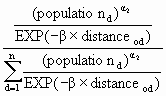

where n is the number of locations in the geographic landscape (e.g., the number of urban places). This specification reveals why the terms K and ₁ of the spatial interaction model are unimportant--they would divide out in this expression. Using Euclidean distance in this formula links to an isotropic geographic landscape, one in which movement in all directions is equally easy.

Disease transmission is assumed to occur through pairwise contacts. The preceding probability expression states the chance that a carrier residing at location o will be paired with a person (carrier or uninfected) at location d. If ₂ = 0 then the probability of a carrier being paired with someone else depends simply on the distance separating their respective locations, distance_od. In this situation, as increases, the probability of interacting defines a circular field surrounding the carrier's location that contracts toward the carrier's location. If equals infinity, then the carrier can infect only other people residing at his/her location. If equals 0, then all other people residing in the geographic landscape have an equal chance of being infected by the carrier, regardless of their respective locations' relative positions.

In contrast, if = 0 then the probability of a carrier being paired with someone else depends simply on the population of the destination location, population_d. In this situation, as ₂ increases, the probability of interacting becomes increasingly hierarchical in nature; the larger a location's population, the greater the chance that a contact will occur. As ₂ increases, the carrier increasingly tends to interact with people residing in the largest urban place(s), regardless of location. If ₂ equals 0, then all other people residing in the geographic landscape have an equal chance of being infected by the carrier, regardless of their respective locations' populations.

Each location has a different set of probabilities. The set of probabilities for location o defines that location's mean information field (MIF). This mean information field allows diffusion to be simulated by converting it to a cumulative set of probabilities. Beginning with the probability assigned to the northwestern-most location, and then moving west-to-east and then north-to-south, locational probabilities can be replace with locational cumulative probabilities. Next these cumulative probabilities can be converted to consecutive intervals, with the lower bound defined by the cumulative probability value for the preceding location and the upper bound being defined by the cumulative probability value for the current location. Suppose the probability in the northwestern-most location is 0.095. Then its interval would be [0, 0.095]. If the cumulative probability value for the location immediately to the east of this first location is 0.235, then this second location's interval would be (0.095, 0.235]. The n intervals, one for each of the n locations, partition the probability interval [0, 1] into n mutually exclusive and collectively exhaustive sub-intervals. Finally, stochastic contact is determined by drawing a uniform pseudo-random number, which is the standard practice, from the interval [0, 1] and allocating it to the location whose interval contains it. Of note is that the sequencing of locations for summing probabilities is irrelevant, and should be selected according to convenience.

Variations on this simulation of diffusion formulation are possible. Reducing the number of susceptible people can be achieved by rescaling the population size. Or, introducing a quarantined region can be achieved by letting the distance parameter be ( + _qI_q), _q >0 and I_q is a binary indicator variable that takes on the value of 1 when a location is quarantined but interacting with a non-quarantined location, and 0 otherwise.

When monitoring the outcome of a simulation experiment, interest is in terms of means, variances, and frequency distributions. Therefore, an experiment needs to be replicated a goodly number of times. When monitoring a single replication, measures of interest include some index of the geographic distribution of the underlying population (perhaps the Moran Coefficient), the rank-size rule parameter, the resulting logistic curve plot, and some space-time measure (perhaps the Knox statistic).

IV. Diffusion waves

An epidemic is the outbreak of some disease in sufficiently large volume, where volume refers to the total number of cases reported during a given length of time coupled with the number of cases per head of population (intensity). Hence brief bursts involving few cases of infection do not constitute an epidemic. Similarly, long strings of small numbers of cases do not constitute multiple epidemics.

The profile of diffusion can be characterized by four phases, each of which describes a distinct stage in a disease epidemic. The primary stage marks the beginning of the diffusion process: an outbreak occurs. This is the ideal time to implement a quarantine The second stage signals the start of the actual disease spread--the upswing in the logistic curve. This is a good time for medical intervention, such as inoculating high-risk populations. Prediction of leaping and creeping--where the disease will appear next--is essential. The third stage involves a condensing of the process: the disease is widespread, and the relative increase in the number of infections is somewhat uniform across the geographic landscape. Medical treatment is common: frequent hospitalization and/or administering of antibiotics. The final stage is that of saturation, where all or nearly all susceptible people have been infected. By this point in time the diffusion process has slowed down, with its eventually cessation on the horizon--the fade-out asymptotic convergence in the logistic curve. This stage is typified by spread throughout the entire geographic landscape. The total cost of the epidemic, in terms of lives and financial resources, can be most accurately assessed at this point in time.

The wave-form of diffusion refers to its space-time depiction. Plotting the spread of a disease across a geographic landscape, using contour maps, uncovers a generalized two-dimensional disease surface that initially increases in both height and extent, but eventually decreasing in height while continuing to increase in extent. Plotting the spread of a disease through time, in the form of a frequency distribution, uncovers alternating peaks and troughs. The timing of these peaks and troughs often occurs with a marked periodicity. Moreover, the wave-form resembles ripples on the surface of a pond created by dropping a stone into the pond. Waves result from interplay between the life cycle of the virus causing a disease and resistance to reinfection.

Cliff et al. supply plots revealing waves of measles epidemics in the U.S., the U.K., Denmark, and Iceland. They observe that in the U.S., which has the largest population, the epidemic cycle was yearly. In the U.K., the epidemic cycle was every two years. In contrast, Iceland has had only eight waves during the reported 25-year period.

V. Applications: diffusion of cholera simulation game

VI. Summary