 [1]
[1]Weighted K-Function
The weighted K-function was developed by Getis (1992) based on the K-function or second order analysis (see K-function). The statistical test is based on the permutations of weighted values at points. For the test, values at points are randomly assigned to the points repeatedly in order to create a confidence envelope.
Input
You’ll be asked to enter the input data file. This file should contain coordinates and the weight for each point (z). You will also be prompted to enter the maximum distance of study, the number of distance increments, and the number of permutations to use in creation of the confidence envelope.
Analysis
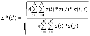
Before performing weighted K-function analysis, K-function analysis should be carried out to determine if the points show a clustered, dispersed, or a CSR pattern. Weighted K-function analysis is then used to determine if the rates or values at each point are clustered, dispersed, or random within the pattern of points. In some sense then, the pattern of weights is independent of location in the simulation. L*(d) includes the interaction of each point with itself, while L(d) does not. An observed L(d) below the minimum expected L(d) indicates that the values are dispersed, whereas an observed L(d) above the maximum expected L(d) indicates that clustering of the values is present at that distance.
Formula
[1]
For![]() ,same as [1] except
,same as [1] except ![]() .
.
A
is the size of the study areaN is the number of points
d
is the distance 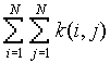 is the number of j points within distance d of all i points
k(i,j) is the weight based on border effects. See the K-function section for
edge correction formulas.
Output
The output file lists the input data file name, the number of points, the minimum and maximum coordinates, the size of the study area, and the following tables showing L(d).
|
Distance (d) |
Observed L(d) |
Minimum L(d) |
Maximum L(d) |
|
: : : |
Limitation
The boundary correction formulas used here are inappropriate for irregular borders. In this program we assume the study area is a regular rectangle or square.
Example
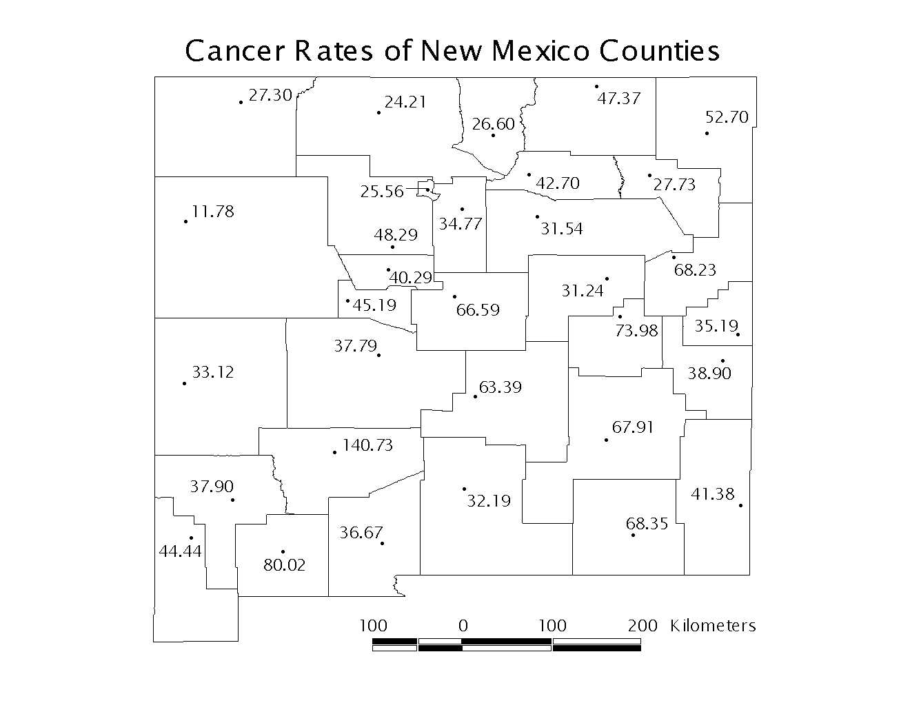
For this example we will consider lung cancer rates in the counties of New Mexico. The data are taken from the National Cancer Institute Biometry Research Group Datasets, and it is available on their website (http://dcp.nci.nih.gov/bb/datasets.html). The total number of cases diagnosed between 1980 and 1989 were divided by the 1985 population estimate to determine the lung cancer rate of each county. The rates are given in cases per 10,000 population. A sample of the input file is shown in Table 1. The statistically unbiased maximum distance is also approximately one half the length of the shortest side of the rectangular study area. New Mexico is approximately 500km per side, so we will set our maximum study distance at 250km. We will choose 25 increments so that we will calculate the observed L(d), observed L*(d), and confidence interval for every 10km. We use 99 permutations to create the confidence envelope in order to test the null hypothesis at the α=0.01 level.
Table 1: Input File
219	338	40.286
27	189	33.124
418	156	76.914
408	538	47.365
534	262	35.186
.	.	.
.	.	.
.	.	.
438	272	73.982
A map of the county seats and their corresponding rates is shown below in Figure 1. Please see the example of K-function analysis where we determined that the county seats are in a dispersed or regular pattern.
Figure 1: New Mexico County Seats
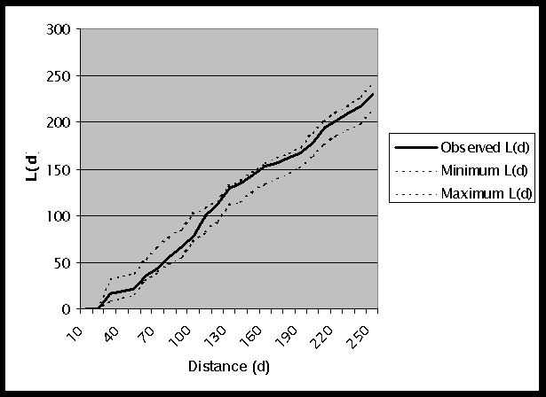
The complete output file for this weighted K-function analysis is shown in Table 2. Remember that L(d) does not include the interaction of each point with itself in the analysis, and this makes L(d) an indicator of the amount of spread of high values around each point. A graph of the results for L(d) is shown in Figure 2. Note that the values found for distances up to 20km are 0.000. This is due to the fact that there are no points within 20km of each other. For the remaining distances, the observed L(d) is within the confidence envelope. This indicates that the cancer rates are distributed in a random pattern within the dispersed pattern of points.
Figure 2: Graph of L(d) Results
L*(d), on the other hand, includes the interaction of each point with itself. A graph of the results of L*(d) is shown in Figure 3. The observed L*(d) values for distances of up to 30km are much higher than d. For all distances the observed L*(d) is within the generated confidence interval. This indicates that, although a particular site may have a high cancer rate, there is not clustering among the sites. We can not reject the null hypothesis of a random pattern of values in the already determined dispersed pattern of points. For further analysis of the same data, see the example using the Gi*(d) statistic.
Figure 3: Graph of L*(d) Results
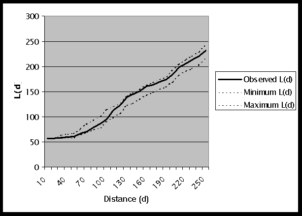
Table 2: Output File
The input data file: nmlung.txt
The total number of points:  32
The minimum x coordinate: 27.000000
The maximum x coordinate: 534.000000
The minimum y coordinate: 30.000000
The maximum y coordinate: 538.000000
The total area: 257556.000000
The maximum search distance: 250.000000
The step size: 10.000000
The number of permutations for the confidence envelope:99
  Distance   Observed L(d)    Minimum L(d)   Maximum L(d)
     10.0000       0.0000       0.0000       0.0000
     20.0000       0.0000       0.0000       0.0000
     30.0000      16.3198       9.7937      32.3642
     40.0000      19.2210      12.4469      35.0250
     50.0000      20.9167      15.2865      37.4224
     60.0000      35.9706      31.3370      52.8135
     70.0000      43.8182      39.8616      66.5759
     80.0000      55.7620      48.6995      76.9947
     90.0000      66.1217      55.2053      85.7109
    100.0000      78.4303      72.2880     101.9169
    110.0000     100.6241      82.6214     109.3578
    120.0000     111.9529      93.3499     115.2715
    130.0000     128.8449     110.9001     131.7032
    140.0000     135.6181     115.2361     139.2102
    150.0000     143.6261     125.4658     146.5212
    160.0000     153.1323     134.4913     156.2502
    170.0000     156.9485     140.0888     162.1014
    180.0000     162.9679     146.3413     167.6751
    190.0000     167.7339     152.2540     173.0551
    200.0000     178.1075     163.3612     188.0481
    210.0000     194.2825     176.8804     201.1089
    220.0000     201.9797     185.9301     210.7177
    230.0000     209.7962     191.8762     218.1049
    240.0000     217.0698     199.5325     227.1929
    250.0000     229.6410     211.8279     241.0012
  Distance   Observed L*(d)   Minimum L*(d)  Maximum L*(d)
     10.0000      56.8175     56.81748     56.81748
     20.0000      56.8175     56.81748     56.81748
     30.0000      59.0261     57.62260     65.07246
     40.0000      59.8592     58.11241     66.38277
     50.0000      60.4029     58.75969     67.62780
     60.0000      66.8667     64.58767     76.86131
     70.0000      71.2226     68.95364     86.52195
     80.0000      78.8365     74.20567     94.46153
     90.0000      86.1867     78.45916    101.41647
    100.0000      95.5894     90.81857    114.91856
    110.0000     113.8188     98.92281    121.31131
    120.0000     123.5644    107.70001    126.46152
    130.0000     138.4758    122.64893    141.03523
    140.0000     144.5554    126.43053    147.79919
    150.0000     151.8038    135.46233    154.43877
    160.0000     160.4817    143.54054    163.34314
    170.0000     163.9851    148.59448    168.73169
    180.0000     169.5316    154.27477    173.88527
    190.0000     173.9398    159.67690    178.87711
    200.0000     183.5794    169.89481    192.86749
    210.0000     198.7149    182.43610    205.13509
    220.0000     205.9553    190.88464    214.20029
    230.0000     213.3296    196.45609    221.18956
    240.0000     220.2093    203.65094    229.80939
    250.0000     232.1351    215.24963    242.94597
References
Getis, A. (1984) Interaction Modeling Using Second-order Analysis, Environment and Planning A 16: 173-183
National Cancer Institute Biometry Research Group Datasets
http://dcp.nci.nih.gov/bb/datasets.html