Nearest Neighbor Analysis

Local K-Function

The local K-function was developed by Getis (1984). It is similar to the global K-function in analysis, but differs in that the local K-function only considers those pairs of points having a given point i as one of its members.

Input

The input data file, which should contain N rows of X, Y coordinates, and W values (a column of 1s).
The maximum distance of study. The statistically unbiased maximum distance is less than the circumradius of the study area, or one-half of the length of the shortest side of a rectangular study area.
The number of increments.
The number of permutations for creating the confidence envelope.
The output file.

Analysis

Like the K-function, the Local K-function is a test of the hypothesis of CSR, and the expected value of L_i(d) is d. Again, the confidence envelope is generated by performing a specified number of simulations. If for any distance the observed L_i(d) falls outside the confidence envelope, the hypothesis of CSR can be rejected at the appropriate significance level. An observed L_i(d) below the envelope indicates that the points are dispersed about point i for distance d. Conversely, an observed L_i(d) above the envelope indicates that the points are clustered about point i for distance d.

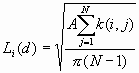
Formula

[1]

where:

A is the study area,

N is the number of points

d is the distance

is the number of points within distance d of point i

is the weight, which includes boundary corrections. The weights are the same as those used in the K-function.

Output

The output file includes the input data file, the total number of points, the minimum and maximum X,Y coordinates, the size of the study area, maximum search distance, number of intervals, and the permutations used in creating the confidence envelope. For each specified distance the following table is printed.

Points	Observed Li(d)	Li(d)-d
1 2 :

Example

For this example we will consider the same data that is used for the Knox statistic example. We are examining cases of an infectious disease during an outbreak. The data includes the X and Y coordinates in meters of each case. A sample of the input data file is shown in Table 1.

Table 1: Input File

X Y Z

138902 58938 1
137625 59262 1
138431 58633 1
138637 58586 1
137738 58994 1
   .     .   .
   .     .   .
   .     .   .
139641 61019 1

The disease is transmitted by a vector that is believed to operate over short distances (less than 35 meters). We will use 35m as our maximum distance of study for this test. A sample of the output is shown in Table 2.

Table 2: Sample Output File

The input data file: cases.dat The total number of points: 294 The minimum x coordinate: 135794.000000 The maximum x coordinate: 141456.000000 The minimum y coordinate: 55984.000000 The maximum y coordinate: 61643.000000 The total area: 32041258.000000 The maximum search distance: 35.000000 The step size: 35.000000 The number of permutation for significance envelope:99 Distance: 35.00 Minimum Li(d): 0.000 Maximum Li(d): 263.852 Point# Observed Li(d) Li(d)-d 1 0.000 -35.000 2 186.572 151.572 3 417.187 382.187

That output file shows that there were a total of 294 cases, and the complete output file contains a L_i(d) value for each point. We have chosen to discuss the output of three key points. These points are shown in the output as points 1,2, and 3.

The L_i(d) for point #1 is 0.00. This indicates that there are no other points within 35m of point #1. We can see that this L_i(d) value is equal to the minimum L_i(d) on the confidence envelope. This indicates that we expect a number of cases not to have a neighboring case within 35m.

The L_i(d) for point #2 is 186.57. This value is well within the confidence envelope. Although there are one or more cases within 35m of point #2, there is not significant clustering of cases around point #2.

The L_i(d) for point #3 is 417.187. This value is well above the maximum L_i(d), and we reject the null hypothesis of a CSR distribution. Recall that a value above the confidence envelope indicates clustering. We can conclude that there is a significant clustering of cases around point #3.

We can see from these three examples that the local K-function gives us an idea of the distribution of points around each point individually.

References

Getis, A, (1984), Interaction Modeling Using Second-order Analysis. Environment and Planning A 16: 173-183

Morrison, Amy C., Getis, Arthur, Santiago, Marilyn, Rigau-Perez, Jose G., and Reiter, Paul (1998). Exploratory Space-Time Analysis of Reported Dengue Cases During an Outbreak in Florida, Puerto Rico, 1991-1992. Am J Trop Med Hyg 58(3): 287-298