 [1]
[1]K-Function
K-function is also called second-order analysis to indicate that the focus is on the variance, or second moment, of pairs of interevent distances. It considers all combinations of pairs of points. It compares the number of observed pairs with the expectation at all distances based on a random spatial distribution of points. The density of points, the borders, and the size of the sample are taken into consideration.
Input
Analysis
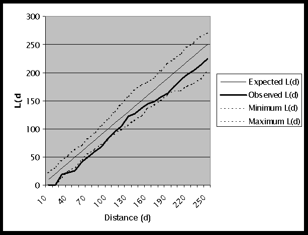
K-function analysis is a test of the hypothesis of CSR. The expected value of L(d) is d. The confidence interval in this analysis is generated by examining the specified number of permutations of randomly generated patterns of N points over the whole study area. If for any distance, the observed L(d) falls above or below the expected L(d) the null hypothesis of CSR can be rejected at an appropriate level of significance. The level of significance is determined by the confidence envelope. An observed L(d) below the envelope indicates that the points are dispersed at that distance, whereas an observed above the envelope indicates that clustering is present at that distance.
Formula
 [1]
[1]
where:
A is the study area,
N is the number of points
d is the distance
 is the number of j points within distance d of all i points
![]() is the weight, which is estimated by
is the weight, which is estimated by
a) If no edge corrections,
![]() in case d(i,j) £ d
in case d(i,j) £ d
![]() otherwise
otherwise
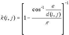
b) If a point i is closer to one boundary than it is to point j, the border correction is employed
 [2]
[2]
where e is the distance to the nearest edge.
c) If a point i is closer to two right angle boundaries than it is to point j, the weighting formula is
 [3]
[3]
where
Output
The output table shows the distance, the observed
L(d), the minimum envelope L(d), and the maximum envelope L(d).|
Distance |
Observed L(d) |
Minimum L(d) |
Maximum L(d) |
|
: : : |
Limitation
The boundary correction formulas used here are inappropriate for irregular borders. In this program we assume the study area is a rectangle or square.
Example
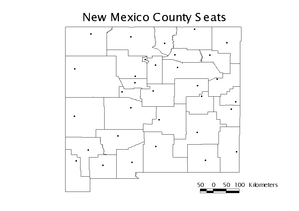
For this example we will consider the distribution of the county seats of New Mexico. A map of New Mexico County Seats is shown in Figure 1.
Figure 1: New Mexico County Seats

There are a total of 32 points in this analysis. The input file is arranged in 32 rows of X, Y coordinates, and W values. Recall, all of the W values are equal to 1. A portion of the input data file is shown in Table 1. New Mexico is approximately 500km per side, so we will set our maximum study distance at 250km. We choose 25 increments so that we will calculate the observed L(d) and confidence interval for every 10km. 99 permutations are used for creating the confidence envelope in order to test the null hypothesis at the a=0.01 level.
Table 1: Input File
X Y W
219 338 1
27 189 1
418 156 1
408 538 1
534 262 1
438 272 1
. . .
. . .
. . .
73 83 1
A graph of the K-function results is shown in Figure 2, and the output file is given in Table 2. The observed L(d) is 0 for 10km and 20km because the closest pair of points is approximately 29km apart. At a distance of 30km, the observed L(d) falls within the generated confidence interval. However, for distances between 40km and 90km the observed L(d) lies outside of the confidence interval. This indicates that we can reject the null hypothesis of CSR. Also, since the observed L(d) is less than the Minimum L(d), this implies that we have a statistically significant dispersed or regular distribution of points.
Figure 2: Graph of K-Function Results

Table 2: Output File
The input data file: nmlung.txt
The total number of points:  32
The minimum x coordinate: 27.000000
The maximum x coordinate: 534.000000
The minimum y coordinate: 30.000000
The maximum y coordinate: 538.000000
The total area: 257556.000000
The maximum search distance: 250.000000
The step size: 10.000000
The number of permutation for significance envelope:99
   Distance    Observed L(d)    Minimum L(d)  Maximum L(d)
   10.00000       0.00000       0.00000      22.26797
   20.00000       0.00000       0.00000      32.45112
   30.00000      18.71896      12.85642      43.69063
   40.00000      22.70875      26.09123      53.86896
   50.00000      26.09549      31.49167      62.89654
   60.00000      41.24103      44.67619      70.69446
   70.00000      50.27186      55.09439      82.33472
   80.00000      59.81204      64.09466      93.76176
   90.00000      68.19498      72.26383     105.88598
  100.00000      83.30301      81.39759     117.37930
  110.00000      94.72131      90.86065     129.75777
  120.00000     104.07702      98.57581     144.20721
  130.00000     122.02663     106.60428     157.24152
  140.00000     126.68748     115.87605     168.35863
  150.00000     136.43529     123.72436     178.46855
  160.00000     144.70865     136.44028     183.43776
  170.00000     149.38940     143.72928     191.86183
  180.00000     156.48955     150.63394     203.29807
  190.00000     163.13176     160.98737     216.70522
  200.00000     175.23454     167.31747     224.97855
  210.00000     187.79141     168.27689     234.22479
  220.00000     196.62003     176.33281     245.17390
  230.00000     204.51863     180.89360     254.47212
  240.00000     212.96201     189.13161     264.24158
  250.00000     224.88269     201.79834     271.39911
References
Boots, Barry N. and Getis, Arthur, 1988, Point Pattern Analysis, Sage University
Paper series on Quantitative Applications in the Social Sciences, series no.07-001, Beverly Hills: Sage Publications
National Cancer Institute Biometry Research Group Datasets
http://dcp.nci.nih.gov/bb/datasets.html