Globals

Global Moran’s I and Global Geary’s c

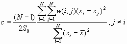
Moran’s I and Geary’s c are well known tests for spatial autocorrelation. They represent two special cases of the general cross-product statistic that measures spatial autocorrelation. Moran’s I is produced by standardizing the spatial autocovariance by the variance of the data. Geary’s c uses the sum of the squared differences between pairs of data values as its measure of covariation. Both of these statistics depend on a spatial structural specification such as a spatial weights matrix or a distance related decline function.

Input

The input data file should contain the X,Y coordinates and the value at each point (x_I).

Input whether you have a spatial weights matrix file.

If you do not have a spatial weights matrix, you’ll be asked to enter the A and m parameters (see below).

You will be asked to enter the maximum distance, the number of steps, and whether you want bands or increments.

Analysis

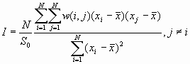
The expected value of Moran’s I is -1/(N-1). Values of I that exceed -1/(N-1) indicate positive spatial autocorrelation, in which similar values, either high values or low values are spatially clustered. Values of I below -1/(N-1) indicate negative spatial autocorrelation, in which neighboring values are dissimilar.

The theoretical expected value for Geary’s c is 1. A value of Geary’s c less than 1 indicates positive spatial autocorrelation, while a value larger than 1 points to negative spatial autocorrelation.

Formula

[1]

[2]

where is the mean of , , , and w(i,j) is the connectivity spatial weight between I and j.

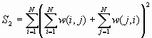
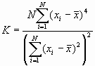
The variances of I and c will differ according to the data model employed. PPA uses a randomization assumption. Under a randomization assumption, the variances of I and c are shown below.

where

The values of Moran’s I and Geary’s c depend on the w(i , j), which are specified by the spatial weighting scheme chosen. In this program, two weighting schemes can be selected:

The w(i,j) are equal to the values in the input N by N matrix taken from the spatial weights matrix file that the user has prepared.

The

, where d(i , j) is the distance between the ith and the jth points; m is a parameter representing the friction of distance selected a priori; A is usually set equal to 1.

In order to evaluate spatial trends in the pattern, sometimes it is necessary to identify spatial autocorrelation at several levels of spatial separation (in the form of a spatial correlogram). In this program, two different correlograms for I and c are available. One type is autocorrelation by bands (Figure 1a) and the other is by cumulative distance increments (Figure 1b).

Figure 1: Correlograms

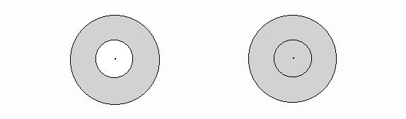
a) bands b) increments

In a, points found in the band represented by the shaded concentric circle are related to the ith point shown in the center. The correlogram shows the relationship of points in each band (from near to far). In b, points found in the shadowed region are related to the ith point at the center. In this case, the correlogram shows the cumulative relationship of points at a series of distances from the i points.

Output for Moran’s I

For each distance range, the program will output

the total number of points,

observed I,

expected I,

the variance,

z value

Output for Geary’s c

For each distance range, the program will output

the total number of points,

observed c,

the variance,

z value

Example

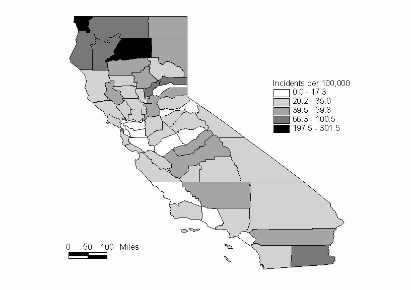
For this example we will consider the distribution of hepatitis rates for the counties of California. The data are taken from the Department of Health Services of the State of California (1999). The rates are given as cases per 100,000 population, and are calculated by using 1998 data over the average population from 1995-1997. The data are shown in Table 1. A map showing the hepatitis rates by county is shown in Figure 2.

Table 1: Reported Hepatitis Rates of California Counties

County	X	Y	Rate
Alameda	195	500	14.4
Alpine	318	560	0
Amador	265	550	12.1
Butte	220	630	52.9
Calaveras	280	530	22.6
Colusa	195	598	23.8
Contra Costa	192	515	12.5
Del Norte	100	790	301.5
El Dorado	260	580	32
Fresno	320	425	53.9
Glenn	180	630	35
Humboldt	90	705	100.5
Imperial	648	56	66.3
Inyo	450	403	29.3
Kern	396	256	41.2
Kings	315	380	21.9
Lake	155	597	39.5
Lassen	270	710	59.2
Los Angeles	436	168	21
Madera	315	455	45
Marin	175	510	20.2
Mariposa	305	485	10.4
Mendocino	125	602	27.5
Merced	285	470	16.6
Modoc	265	765	59.8
Mono	380	515	31.6
Monterey	212	415	26.6
Napa	185	545	23.8
Nevada	255	610	13.8
Orange	468	112	17.3
Placer	270	595	50.8
Plumas	272	660	34.6
Riverside	600	120	46.5
Sacramento	235	548	43.1
San Benito	220	430	25
San Bernadino	584	216	33.7
San Diego	544	52	22.4
San Fransisco	185	503	78.2
San Joaquin	236	520	30.5
San Luis Obispo	272	260	11.8
San Mateo	190	490	26.6
Santa Barbara	300	200	24.4
Santa Clara	202	475	14.8
Santa Cruz	200	450	27.8
Shasta	197	712	197.5
Sierra	275	630	78.4
Siskiyou	180	782	75.9
Solano	192	540	23.6
Sonoma	170	535	24.6
Stanislaus	265	491	26.8
Sutter	210	590	32.6
Tehama	193	680	58.3
Trinity	140	702	75
Tulare	365	385	30.3
Tuolumne	303	515	20.7
Ventura	372	176	16.2
Yolo	205	570	30.6
Yuba	228	604	79.8

Figure 2: Hepatitis Rates of California Counties in 1998 (per 100,000 pop.)

For this example we will use the following weighting scheme:

,thus A = 1 and m = 2

Both Moran’s I and Geary’s c results are shown in Table 2. The Moran’s I and Geary’s c statistics are calculated for 50-mile increments from 50 to 250 miles. For each of these increments, the Geary’s c is less than 1, and the Moran’s I is greater than the expected value. These results indicate that there is positive spatial autocorrelation. However, none of the Z-values are significant at the a =0.05 level, and we can not reject the null hypothesis of a random distribution of hepatitis rates. From this analysis using Moran’s I and Geary’s c, we must conclude that there is not significant spatial autocorrelation.

Table 2: Output

The input data file: hep.dat

The total number of points: 58
Distance Moran's I Expected I Variance Z-value
50.0000 0.0319 -0.0175 0.0172 0.3776
100.0000 0.0638 -0.0175 0.0095 0.8365
150.0000 0.0704 -0.0175 0.0077 0.9995
200.0000 0.0673 -0.0175 0.0072 0.9980
250.0000 0.0652 -0.0175 0.0070 0.9875
The input data file: hep.dat
The total number of points: 58
Distance Geary's c Variance Z-value
50.0000 0.27181 0.700783 -0.86986
100.0000 0.28573 0.455953 -1.05779
150.0000 0.29893 0.391380 -1.12063
200.0000 0.31507 0.365535 -1.13287
250.0000 0.33074 0.354542 -1.12398

References

Cliff, A.D. and Ord, J.K. (1973) Spatial Autocorrelation, Pion: London

Cliff, A.D. and Ord, J.K. (1981) Spatial Processes: Models and Applications, Pion: London

State of California Department of Health Services (March 1999). 1998 Report Health Data Summaries for California Counties