Nearest Neighbor Analysis

Refined Nearest Neighbor Analysis

Refined nearest neighbor analysis involves comparing the complete distribution function of the observed nearest neighbor distances, F(d_i £ r), with the distribution function of the expected nearest neighbor distances for complete spatial randomness (CSR), P(d_i £ r). CSR is generated by means of two assumptions: 1) that all places are equally likely to be the recipient of a case (event) and 2) all cases are located independent of one another. This procedure differs from Nearest Neighbor Analysis in that the basis for border correction is taken from literature that recommends that a "guard area" represent an objective view of border conditions. (see Boots and Getis 1988)

Input

You’ll be asked to enter the input data file, which should contain N rows of X, Y coordinates, and W values. Make all W values equal to 1, representing points.

Analysis

Refined nearest neighbor analysis is used to test the null hypothesis of CSR. If for each distance, F(d_i £ r) > P(d_i £ r), a clustered pattern is indicated, whereas P(d_i £ r) < P(d_i £ r) indicates a regular pattern. The largest absolute distance (d_r) between the F(d_i £ r) and the P(d_i £ r) is found. The significance of d_ris then measured using a Monte Carlo test. If for this significant value, d_r, F(d_i £ r) > P(d_i £ r) clustering is implied.

Formula

F(d_i £ r) is obtained by taking the nearest neighbor distances, d_i, and the nearest distances to study boundary, u_i, for each point i. The program ranks d_i from the smallest to the largest. For every distance of interest, r, the program counts the number of points n₁ for which d_i £ r, and the number of points n₂ for which u_i < r < d_i. The observed proportion of the nearest neighbor distances less than or equal to some chosen distance r is decided by equation [1].

[1]

where N is the total number of points

The proportion of expected nearest neighbor distances less than or equal to r for an unbounded CSR pattern is:

[2]

Where:

e is the constant 2.178283

p is the constant 3.141593

r is the specified distance

l is the estimated point density (N/A)

c) d_r

[3]

where max | | means the largest absolute value obtained for corresponding values of r

Output

The output file includes three parts: the first part lists a) the input data file, b) the total number of points, c) the minimum and maximum of X, and Y coordinates, and d) the size of study area. The second part is a table in the following form:

r (distance)	n1 (observed number of points for which d_i £ r)	n2 (observed number of points for which u_i< r < d_i)	F(r) (observed proportion P(d_i £ r))	P(r) (expected proportion P(d_i £ r))	\|F(r) - P(r)\| (absolute value of the difference)
: : :

Limitation

In this program, the study area is a regular rectangle or square. Area (A) is calculated by (Xmax – Xmin) * (Ymax – Ymin).

Example

For this example of Refined Nearest Neighbor Analysis we will consider Figure 1, which shows incidents of larynx cancer the Chorley and South Ribble area of Lancashire, England. This data is available on Peter Diggle’s web site (http://www.maths.lancs.ac.uk/~diggle/pointpatterns/Datasets/). The null hypothesis (H₀) is that the points are in a CSR pattern. The area used in the analysis is shown by the rectangle in Figure 1. The Xmin, Ymin, Xmax, and Ymax are shown in the output file (Table 2).

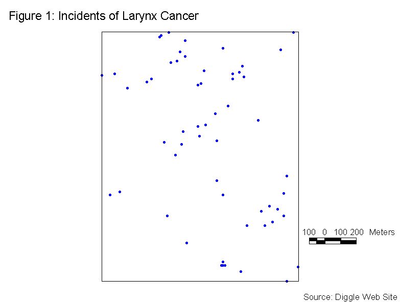
There are a total of 58 points in this sample. The input file is arranged in 58 rows of X, Y coordinates, and W values. For Refined Nearest Neighbor Analysis, all of the W values are set to 1. A portion of the input data file is shown in Table 1.

Table 1: Sample of input data file

X Y Z 35320 42800 1 35310 42230 1 34910 41850 1 35260 42080 1 35300 42150 1 35230 42660 1 36000 42850 1 34960 42500 1 35690 42570 1 . . . . . . . . . 34850 41830 1

For these data, table 2 shows that d_r is 0.371. The results of the Monte Carlo test, a simulation run 99 times, indicates that this is significant at the 0.01 level. The null hypothesis of CSR can be rejected for a =0.01. This d_r occurs at a distance of 63.246 meters, where the F(d_i £ r) > P(d_i £ r). This implies that the pattern is clustered.

Table 2: Output File

The input data file: d:\ppa\lardat.txt The total number of points: 58 The minimum x coordinate: 34800.000000 The maximum x coordinate: 36030.000000 The minimum y coordinate: 41290.000000 The maximum y coordinate: 42850.000000 The total area: 1918800.0000

r, n1, n2, F(r), P(r), |F(r) - P(r)| 0.000 2 12 0.043 0.000 0.043 10.000 6 12 0.130 0.009 0.121 14.142 8 12 0.174 0.019 0.155 20.000 9 12 0.196 0.037 0.158 22.361 11 12 0.239 0.046 0.193 30.000 13 12 0.283 0.082 0.201 36.056 15 12 0.326 0.116 0.210 41.231 18 12 0.391 0.149 0.242 42.426 21 12 0.457 0.157 0.299 44.721 22 12 0.478 0.173 0.305 50.990 24 12 0.522 0.219 0.303 53.852 28 11 0.596 0.241 0.355 56.569 29 11 0.617 0.262 0.355 58.310 30 11 0.638 0.276 0.362 60.828 31 11 0.660 0.296 0.363 63.246 33 10 0.688 0.316 0.371 80.623 38 8 0.760 0.461 0.299 82.462 39 8 0.780 0.476 0.304 92.195 40 8 0.800 0.554 0.246 94.340 41 8 0.820 0.571 0.249 98.489 43 8 0.860 0.602 0.258 106.301 44 8 0.880 0.658 0.222 107.703 46 6 0.885 0.668 0.217 110.000 47 6 0.904 0.683 0.221 111.803 48 5 0.906 0.695 0.211 114.018 51 3 0.927 0.709 0.218 120.416 52 3 0.945 0.748 0.198 136.015 54 1 0.947 0.827 0.120 162.788 55 0 0.948 0.919 0.029 208.087 57 0 0.983 0.984 0.001 210.238 58 0 1.000 0.985 0.015 The Maximum d(r): 0.371 This d(r) is at 0.010 signficance level

References

Boots, Barry N. and Getis, Arthur, 1988, Point Pattern Analysis, Sage University

Paper series on Quantitative Applications in the Social Sciences, series no.07-001, Beverly Hills: Sage Publications

Diggle, Peter J., 1990, "A Point Process Modelling Approach to Raised Incidence of a Rare Phenomenon in the Vicinity of a Prespecified Point." Journal of the Royal Statistical Society A, 153(3), 349-362