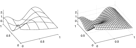
At left the curvemesh; at right its interpolant. |
|
At left the curvemesh; at right its interpolant. |
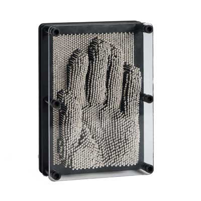
A few years ago a gift named "Pinpressions" appeared under our family's Christmas tree:
 |
 |
The designers of Pinpressions were very sensible, and, in order to pack the pins in better, staggered rows and columns like a honeycomb. Imagine if you will that they were not so intelligent! Imagine that the rows and columns of pins fall on a regular grid. Then we could think of Pinpressions as a 3-D plotter on a gridded domain.
Now a matrix captures all the information in this plot, if we associate the rows of the matrix with rows of pins (which lie along the x-axis of a Cartesian coordinate system); the columns of the matrix with columns of pins (the y-axis of the coordinate system); and the heights of the pins, or z-coordinates, we associate with the components of the matrix aij.
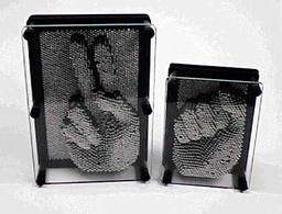
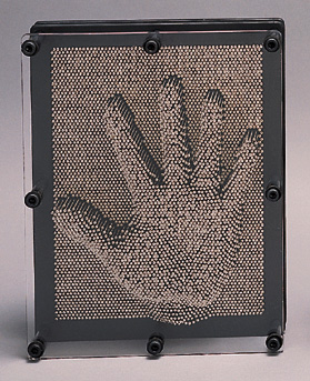
In this sense, we also consider Pinpressions to be a matrix plotter. The zero matrix represents the "default" position of the pins: Pinpressions with all pins pushed in (the heights of the pins are all zero). We can generate a plot represented by a more complex matrix by "pressing the flesh":
In sum: we can think of this 3-D point data set as a matrix, where the rows and columns have a physical position assigned to them.
Cliff has been interested in this dual, Pinpressions-type representation of a matrix for a long time. He dreams of a "function-box", which we can think of as Pinpressions with little motors to drive the heights of the pins up and down. A function-box user could plot a function of two-variables by presenting its formula to the function-box, which would then position the pins according to its graph.
And so we would represent functions by 3-D point data sets.
Now we can turn this idea on its head: Cliff's goal is to go from
Today we begin by considering the process of going from
Given matrix A can we create a function f such that
That is, can we find a function which interpolates A?
We have developed a simple technique for doing so, based on 1-D interpolation and the Singular Value Decomposition, a process which we will describe in a moment. From this method it is a short step to fitting curvemeshes, as we will show below. Let's have a look! But first of all,
|
At left the curvemesh; at right its interpolant. |
The curves of the mesh are given by (x,yj,gj(x)) and (xi,y,hi(y)).
Note: gj(xi) = hi(yj) = aij
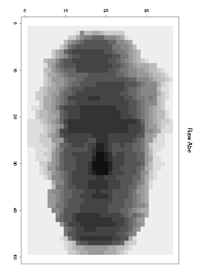
Here is a matrix of data as it might be read off of the Pinpressions function box (with Abraham Lincoln's face substituting for the hand in the images above). The color (or shade) represents the height of the pins: |
||
 |
||
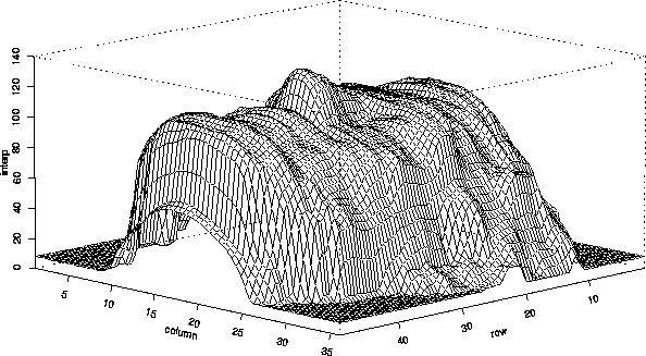
As mentioned, we developed a simple method of create a function from a matrix. Here's Abe again, only now as the graph of a function of two variables: |
||
 |
||
This matrix interpolation process is based on interpolation of simple (rank-one) matrices: matrices which can be written as the outer-product of two vectors. For example,
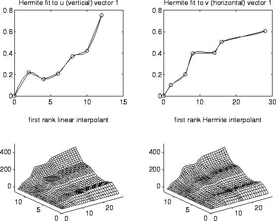
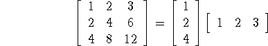 Each column is a multiple of any other column; similarly for the rows. Below we see how matrix interpolation works for a rank-one matrix which is associated with a gridded data set: |
||
 |
||
The two resulting surfaces, drawn in the bottom panels above, indicate that we have a lot of freedom when it comes to "skinning a matrix" (that is, creating a skin for a matrix).The Singular Value Decomposition simply states that any matrix can be written as a sum (in an optimal way) of these simple, rank-one matrices. To interpolate Abe to create the Abe function, we decomposed the Abe matrix, interpolated each rank-one matrix, and simply added these rank-one interpolants. |
||
Having successfully interpolated matrices, we next proceeded to consider the problem of boundary conditions: could we choose our interpolation method so as to match boundary curves? |
||
 |
||
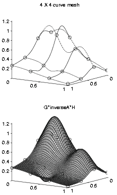
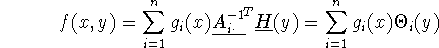
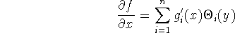
Yes! But, moreover, we discovered that we had enough freedom to match r row and r column curves, where r is the rank of the matrix A. Thus, if A were square and full-rank (and hence invertible), we deduced that we could interpolate a square curvemesh, and produced the formula
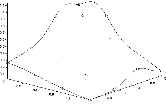
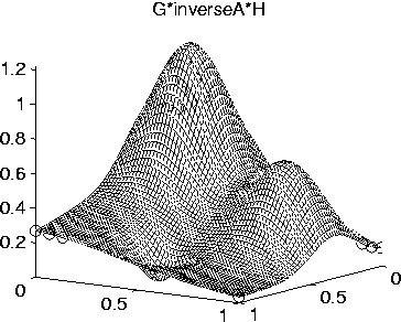
for the interpolant. The simplicity of this formulation came as some surprise! Here is an example with a 4x4 mesh: |
||
|
||
Using this formulation, however, it's clear that there are no degrees of freedom left: once G and H are prescribed, f is fully prescribed.
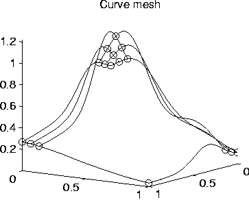
As we see in the following image, different choices of G and H may still give rise to the same function: |
||
|
||
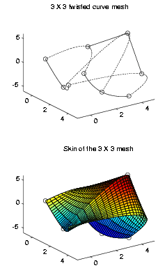
This has to do with the relative simplicity of the Franke function mentioned above.You may want to get fancy, and consider twisted curvemeshes - no problem with our method: |
||
 |
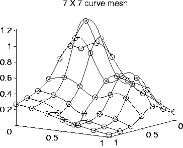
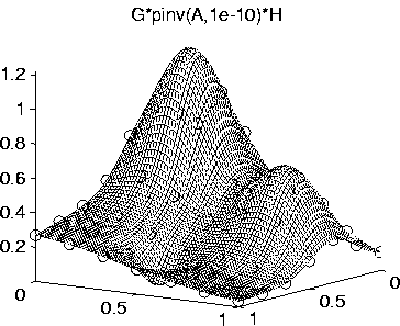
And so ends our brief tour of curvemesh interpolation. There are several points we might mention to bring our presentation to a close:
Example: as mentioned earlier, Franke's function only requires 4 curves to reconstitute it. Here we provide 7, but the method still works (and only uses 4 of the 7 curves!).