You are using Rweb1.04 on the server at www.nku.edu
Rweb:>
Rweb:> ##
Rweb:> ############## RClimate Script: Mauna Loa Monthly CO2 ###################################
Rweb:> ## ##
Rweb:> ## Download and process Monthly CO2 Data File ##
Rweb:> ## Developed by D Kelly O'Day to demonstrate use of source() function for climate data ##
Rweb:> ## http:chartsgraphs.wordpress.com 1/16/10 ##
Rweb:> ## Revised 12/15/14; removed personal info for posting ##
Rweb:> ## Contributions from Andy Long: ##
Rweb:> ## Revised 3/2015; Added models (quadratic and exponential) ##
Rweb:> ############################################################################################
Rweb:> ##
Rweb:> library(plyr);
Rweb:> library(reshape);
Rweb:> ##
Rweb:> par(las=1);
Rweb:> par(ps=10)
Rweb:>
Rweb:> ## STEP 1: SETUP
Rweb:> ##
Rweb:> url <- "ftp://aftp.cmdl.noaa.gov/products/trends/co2/co2_mm_mlo.txt"
Rweb:> link <-file("/var/www/html/data/Rweb/RClimate/data/co2_mm_mlo.txt")
Rweb:>
Rweb:> ## STEP 2: READ DATA
Rweb:> CO2_data <- read.table(link,sep="",row.names=NULL,header=F,
+ colClasses = rep("numeric", 7), skip=74,
+ comment.char = "#", na.strings = -99.99)
Rweb:> names(CO2_data) <- c("Yr", "Mo", "Mo_Yr", "CO2", "Trnd", "X", "dys")
Rweb:>
Rweb:> ## STEP 3: Determine Month, Year for last reading
Rweb:> nrows <- nrow(CO2_data) # Find number of data rows
Rweb:> mo <- CO2_data[nrows,2] # Find last month of data
Rweb:> yr <- CO2_data[nrows,1] # Find last year od data
Rweb:> lco2 <- CO2_data[nrows,4] # Find last CO2 reading
Rweb:>
Rweb:> ## STEP 4: CREATE PLOT
Rweb:> ## Set Chart Parameters
Rweb:> par(las=1);par(ps = c(15));par(pin = c(6,3))
Rweb:> par(oma=c(3.5,1,4,1)); par(mar=c(2,4,0,0))
Rweb:> ## Make Basic Plot
Rweb:> plot_func <- function() {
+ plot(CO2 ~ Mo_Yr, CO2_data,
+ ylim = c(300,440),
+ xlim = c(1958, yr+2),
+ type="l", xaxs = "i", yaxs="i",
+ col = "black", cex.main=1.5, cex.axis = 1, cex.lab = 1,
+ xlab = "",
+ ylab = expression(paste(CO[2] - ppmv)))
+ ## Add last point & Yr - month note
+ points(CO2_data[nrows,3], lco2, type = "p",pch=16, col = "red")
+ points(1959, 395, type = "p",pch=16, col = "red")
+ abline(h=400, col="grey")
+ text(1960, 303, paste("Source NOAA: ", url), adj=0, cex = .8)
+ ## Plot Annotation
+ mo_names <- c("Jan,", "Feb,", "Mar,", "Apr,", "May,", "June,", "July,", "Aug,", "Sept,", "Oct,", "Nov,", "Dec,")
+ thru <- paste(mo_names[mo],yr, "- ", lco2, " ppmv") # Note on last data point
+ text(1960,395, thru, cex=0.8, adj=0)
+ points(c(1958,1960), c(390,390), type = "l", col = "red")
+ Title <- expression(paste("C", O[2], " (ppmv)Trends Since 1958, Mauna Loa, Hawaii"))
+ mtext(Title, 3,2, outer = TRUE)
+ mtext(paste("Data Updated Through", mo_names[mo], yr), 3,1, outer = TRUE, cex = 0.85)
+ mtext("Andy Long and D Kelly O'Day", 1,1, adj = 0, cex = 0.8, outer=TRUE)
+ mtext(format(Sys.time(), "%m/%d/%Y"), 1, 1, adj = 1, cex = 0.8, outer=TRUE)
+ }
Rweb:> plot_func()
Rweb:>
Rweb:> ######################################################################
Rweb:> ##
Rweb:> ## Add a quadratic trend model (use the year 2000 as the baseline):
Rweb:> ##
Rweb:> ######################################################################
Rweb:> date <- CO2_data[,3]-2000
Rweb:> date2 <- date^2
Rweb:> avgCO2 <- CO2_data[,4]
Rweb:> Keeling <- data.frame(avgCO2,date,date2)
Rweb:> ## http://stackoverflow.com/questions/4862178/remove-rows-with-nas-in-data-frame
Rweb:> ## drop out the data that's missing -- won't be useful in modeling, anyway....
Rweb:> Keeling <- na.omit(Keeling)
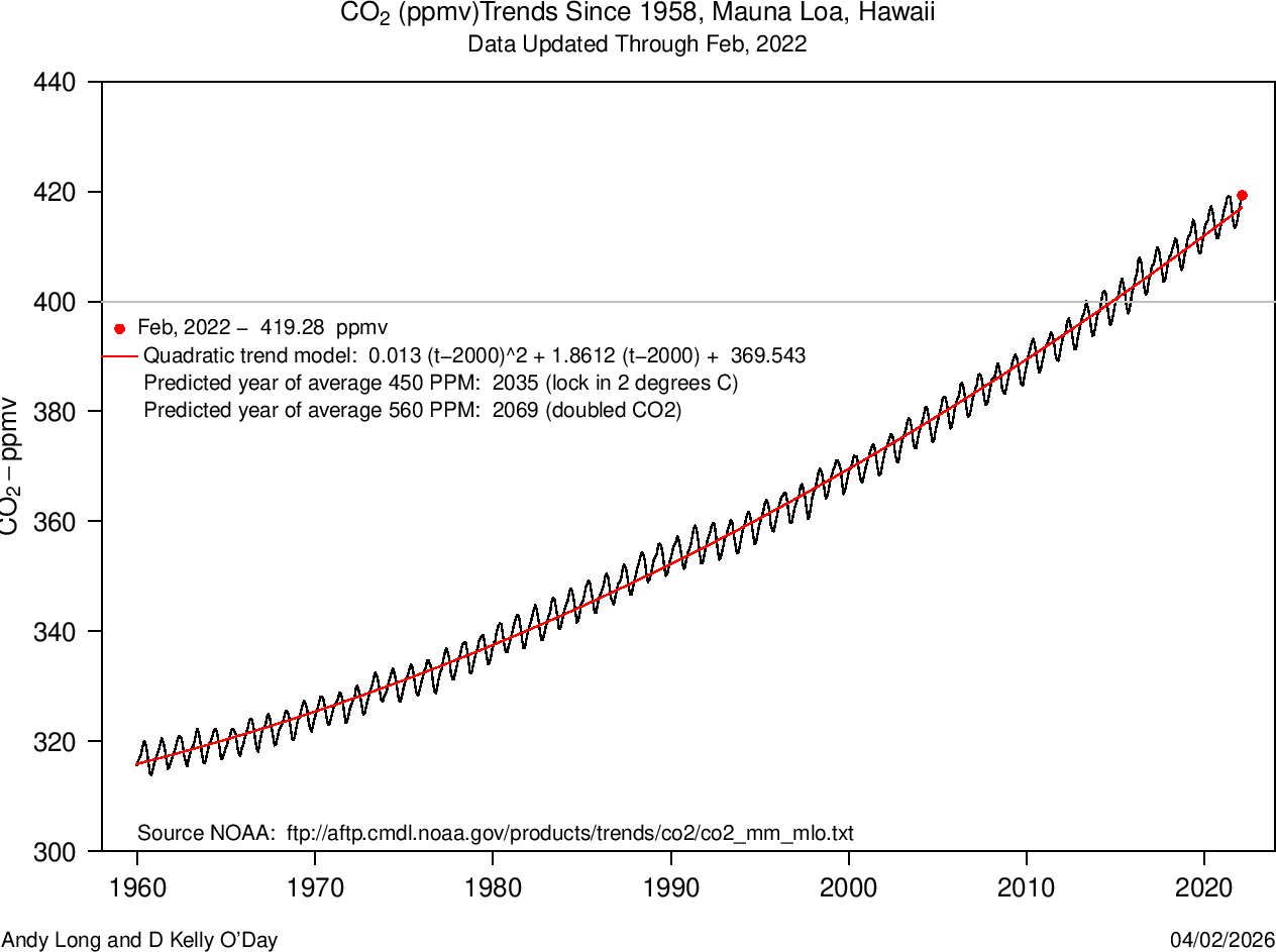
Rweb:> q_m <- lm(avgCO2 ~ date + date2, data=Keeling)
Rweb:> summary(q_m)
Call:
lm(formula = avgCO2 ~ date + date2, data = Keeling)
Residuals:
Min 1Q Median 3Q Max
-4.9060 -1.8254 0.1105 1.7940 4.7724
Coefficients:
Estimate Std. Error t value Pr(>|t|)
(Intercept) 3.695e+02 1.146e-01 3225.38 <2e-16 ***
date 1.861e+00 6.830e-03 272.51 <2e-16 ***
date2 1.300e-02 2.837e-04 45.84 <2e-16 ***
---
Signif. codes: 0 ‘***’ 0.001 ‘**’ 0.01 ‘*’ 0.05 ‘.’ 0.1 ‘ ’ 1
Residual standard error: 2.24 on 744 degrees of freedom
Multiple R-squared: 0.9943, Adjusted R-squared: 0.9943
F-statistic: 6.478e+04 on 2 and 744 DF, p-value: < 2.2e-16
Rweb:> coefs <- coefficients(q_m)
Rweb:> a <- coefs[3]
Rweb:> b <- coefs[2]
Rweb:> c <- coefs[1]
Rweb:> points(Keeling$date+2000,predict(q_m),type="l",col="red")
Rweb:>
Rweb:> ## describe model:
Rweb:> thru <- paste(" Quadratic trend model: ",round(a,4),"(t-2000)^2 +",round(b,4),"(t-2000) + ",round(c,4))
Rweb:> text(1960,390, thru, cex=0.8, adj=0)
Rweb:>
Rweb:> ## find out when the quadratic will hit 450: i.e., find roots of q(x)=450, or ax^2+bx+c-450=0:
Rweb:> c <- coefs[1] - 450
Rweb:> root <- (-b+sqrt(b^2-4*a*c))/(2*a) + 2000
Rweb:> thru <- paste(" Predicted year of average 450 PPM: ",round(root), "(lock in 2 degrees C)")
Rweb:> text(1960,385, thru, cex=0.8, adj=0)
Rweb:>
Rweb:> ##
Rweb:> ## "For the past 10,000 years, the amount of CO2 in the atmosphere stayed
Rweb:> ## almost constant at about 280 ppm. Then, in about 1750 the picture changed."
Rweb:> ## Eggleton, R. A. Eggleton, Tony (2013). A Short Introduction to Climate
Rweb:> ## Change. Cambridge University Press. p. 52:
Rweb:> ##
Rweb:> ## https://books.google.co.uk/books?id=jeSwRly2M_cC&pg=PA52&lpg=PA52&dq=280
Rweb:> ## found in
Rweb:> ## https://en.wikipedia.org/wiki/Carbon_dioxide_in_Earth%27s_atmosphere
Rweb:> ##
Rweb:> ## find out when the quadratic will hit 560: i.e., find roots of q(x)=560, or ax^2+bx+c-560=0:
Rweb:> c <- coefs[1] - 560
Rweb:> root <- (-b+sqrt(b^2-4*a*c))/(2*a) + 2000
Rweb:> thru <- paste(" Predicted year of average 560 PPM: ",round(root), "(doubled CO2)")
Rweb:> text(1960,380, thru, cex=0.8, adj=0)
Rweb:>
Rweb:> ######################################################################
Rweb:> ##
Rweb:> ## Let's try an exponential trend model:
Rweb:> ##
Rweb:> ######################################################################
Rweb:> ##
Rweb:> plot_func()
Rweb:> ##
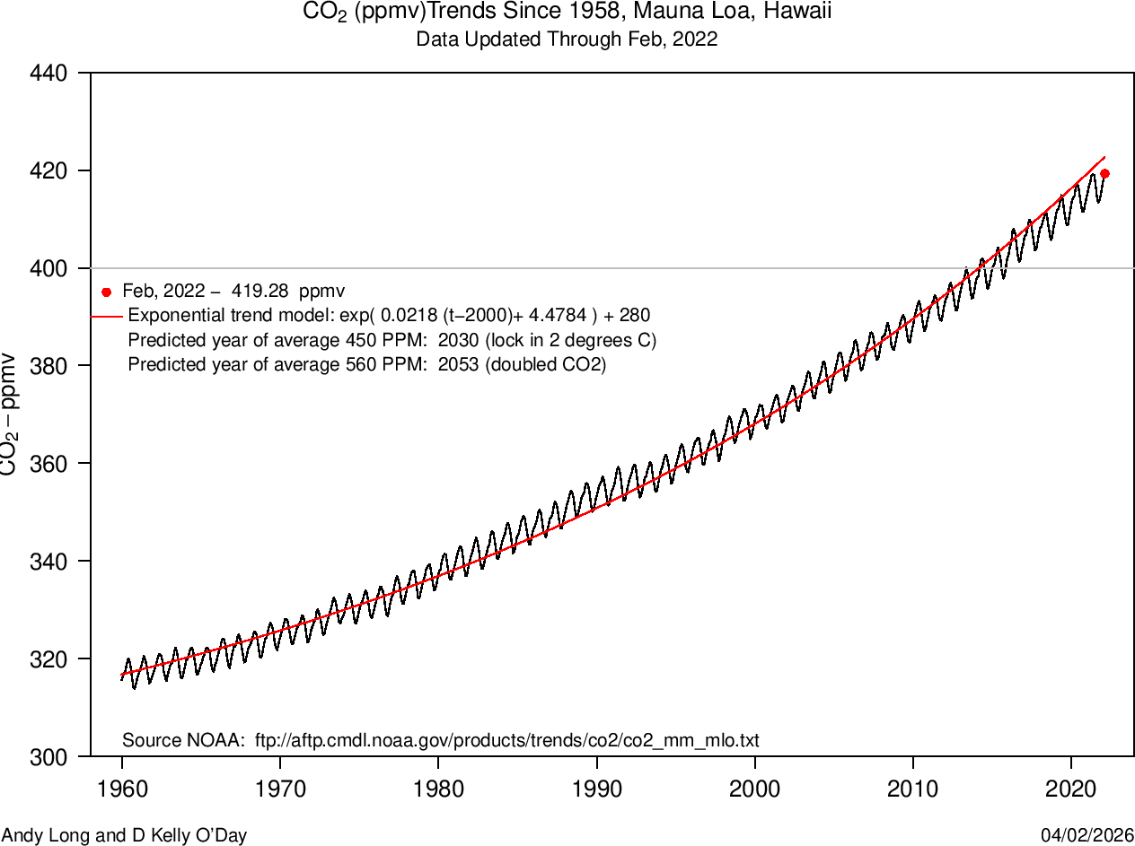
Rweb:> historical <- 280 ## (modelling exponential departure from the long-term historical trend of roughly 280 ppm)
Rweb:> ln_avgCO2 <- log(avgCO2 - historical)
Rweb:> Keeling <- data.frame(ln_avgCO2,avgCO2,date)
Rweb:> ## http://stackoverflow.com/questions/4862178/remove-rows-with-nas-in-data-frame
Rweb:> ## drop out the data that's missing -- won't be useful in modeling, anyway....
Rweb:> Keeling <- na.omit(Keeling)
Rweb:> q_m <- lm(ln_avgCO2 ~ date, data=Keeling)
Rweb:> summary(q_m)
Call:
lm(formula = ln_avgCO2 ~ date, data = Keeling)
Residuals:
Min 1Q Median 3Q Max
-0.11390 -0.02590 -0.00006 0.02854 0.08392
Coefficients:
Estimate Std. Error t value Pr(>|t|)
(Intercept) 4.478e+00 1.581e-03 2832 <2e-16 ***
date 2.181e-02 7.874e-05 277 <2e-16 ***
---
Signif. codes: 0 ‘***’ 0.001 ‘**’ 0.01 ‘*’ 0.05 ‘.’ 0.1 ‘ ’ 1
Residual standard error: 0.03868 on 745 degrees of freedom
Multiple R-squared: 0.9904, Adjusted R-squared: 0.9904
F-statistic: 7.67e+04 on 1 and 745 DF, p-value: < 2.2e-16
Rweb:> coefs <- coefficients(q_m)
Rweb:> points(Keeling$date+2000,exp(predict(q_m)) + historical,type="l",col="red")
Rweb:> ## describe model:
Rweb:> thru <- paste(" Exponential trend model: exp(",round(coefs[2],4),"(t-2000)+",round(coefs[1],4),") +",historical)
Rweb:> text(1960,390, thru, cex=0.8, adj=0)
Rweb:>
Rweb:> a <- coefs[2]
Rweb:> b <- coefs[1]
Rweb:> root <- (log(450 - historical) - b)/a + 2000
Rweb:> thru <- paste(" Predicted year of average 450 PPM: ",round(root), "(lock in 2 degrees C)")
Rweb:> text(1960,385, thru, cex=0.8, adj=0)
Rweb:>
Rweb:> root <- (log(560 - historical) - b)/a + 2000
Rweb:> thru <- paste(" Predicted year of average 560 PPM: ",round(root), "(doubled CO2)")
Rweb:> text(1960,380, thru, cex=0.8, adj=0)
Rweb:>
Rweb:>
Rweb:>